【 Notes 】Best linear unbiased estimator(BLUE) approach for time-of-arrival based localisation-白红宇

【 Notes 】Best linear unbiased estimator(BLUE) approach for time-of-arrival based localisation

阅读量：2027 次

发布时间：2019-04-28

本文共 10998 字，大约阅读时间需要 36 分钟。

Abstract

A common technique for source localisation is to utilise the time-of-arrival (TOA) measurements between the source and several spatially separated sensors. The TOA information defines a set of circular equations from which the source position can be calculated with the knowledge of the sensor positions.

源定位的常用技术是利用源和若干空间分离的传感器之间的到达时间（TOA）测量。 TOA信息定义了一组圆形方程，从中可以利用传感器位置的知识计算源位置。

Apart from nonlinear optimisation, least squares calibration (LSC) and linear least squares (LLS) are two computationally simple positioning alternatives which reorganise the circular equations into a unique and non-unique set of linear equations, respectively. As the LSC and LLS algorithms employ standard least squares (LS), an obvious improvement is to utilise weighted LS estimation.

除了非线性优化之外，最小二乘校准（LSC）和线性最小二乘（LLS）是两种计算上简单的定位选择，它们将圆形方程分别重新组织成一组唯一且非唯一的线性方程组。由于LSC和LLS算法采用标准最小二乘（LS），因此明显的改进是利用加权LS估计。

In the paper, it is proved that the best linear unbiased estimator (BLUE) version of the LLS algorithm will give identical estimation performance as long as the linear equations correspond to the independent set. The equivalence of the BLUE-LLS approach and the BLUE variant of the LSC method is analysed. Simulation results are also included to show the comparative performance of the BLUE-LSC, BLUE-LLS, LSC, LLS and constrained weighted LSC methods with Crame´r–Rao lower bound.

在本文中，证明了LLS算法的最佳线性无偏估计（BLUE）版本将给出相同的估计性能，只要线性方程对应于独立集合。分析了BLUE-LLS方法与LSC方法的BLUE变体的等价性。还包括模拟结果，以显示BLUE-LSC，BLUE-LLS，LSC，LLS和具有Crame'r-Rao下限的约束加权LSC方法的比较性能。

注：最佳线性无偏估计(best linear unbiased estimator)（BLUE）

Introduction

Source localisation using measurements from an array of spatially separated sensors has been an important problem in radar, sonar, global positioning system [1], mobile communications [2], multimedia [3] and wireless sensor networks [4]. One commonly used location-bearing parameter is the time-of-arrival (TOA) [2, 4], that is, the one-way signal propagation or round trip time between the source and sensor. For two-dimensional positioning, each noise-free TOA provides a circle centred at the sensor on which the source must lie. By using M >= 3 sensors, the source location can be uniquely determined by the intersection of circles. In practice, the TOA measurements

are noisy, which implies multiple intersection points and thus they are usually converted into a set of circular equations, from which the source position is estimated with the knowledge of the signal propagation speed and sensor array geometry.

Commonly used techniques for solving the circular equations include linearisation via Taylor-series expansion [5] and steepest descent method [6]. Although this direct approach can attain optimum estimation performance, it is computationally intensive and sufficiently precise initial estimates are required to obtain the global solution. On the other hand, an alternative approach, which allows real-time

computation and ensures global convergence is to reorganise the nonlinear equations into a set of linear equations by introducing an extra variable that is a function of the source position. It is noteworthy that this idea is first introduced in [7, 8] for time-difference-of-arrival (TDOA) based localisation.

解决圆形方程的常用技术包括通过泰勒级数展开[5]和最速下降法[6]的线性化。尽管这种直接方法可以获得最佳估计性能，但它是计算密集型的，并且需要足够精确的初始估计来获得全局解。另一方面，允许实时计算并确保全局收敛的替代方法是通过引入作为源位置的函数的额外变量将非线性方程组织成一组线性方程。值得注意的是，这个想法首先在[7,8]中引入，用于基于时间差（TDOA）的定位。

The linear equations can then be solved straightforwardly by using least squares (LS) and the corresponding estimator is referred to as the least squares calibration (LSC) method [9], or by eliminating the common variable via subtraction of each equation from all others, which is referred to as the linear least squares (LLS) estimator [10, 11].

然后可以通过使用最小二乘（LS）直接求解线性方程，并且相应的估计器被称为最小二乘校准（LSC）方法[9]，或者通过从所有其他方程中减去每个方程来消除公共变量，这被称为线性最小二乘（LLS）估计[10,11]。

In this work, we will focus on the relationship development between the best linear unbiased estimator (BLUE) [12] versions of the LSC and LLS algorithms. Our contributions do not lie on new positioning algorithm development as the BLUE technique for localisation applications has already been proposed in the literature [13]. Our major findings include

在这项工作中，我们将重点关注LSC和LLS算法的最佳线性无偏估计（BLUE）[12]版本之间的关系开发。我们的贡献不在于新的定位算法开发，因为文献中已经提出了用于定位应用的BLUE技术[13]。我们的主要发现包括

(i) all BLUE realisations of the LLS algorithm have identical estimation performance as long as the (M -1) linear equations correspond to the independent set [10].

（i）所述LLS算法的所有实现中BLUE具有相同的估计性能，只要该（M-1）的线性方程组对应于独立组[10]。

(ii) The covariance matrices of the position estimates in the BLUE-LLS scheme with the independent set and the BLUE version of the LSC algorithm are identical.

（ii）BLUE-LLS方案中具有独立集合的位置估计的协方差矩阵和LSC算法的蓝BLUE版本是相同的。

By comparing with Crame ´r–Rao lower bound (CRLB) for TOA-based localisation [14], it is then shown that they are suboptimal estimators, and this result is different from the iterative BLUE estimator of [13], which gives maximum likelihood estimation performance.

通过与基于TOA的定位的Crame'r-Rao下界（CRLB）进行比较[14]，然后表明它们是次优估计，并且该结果与[13]的迭代BLUE估计不同，其给出最大似然估计性能。

(iii) Among the BLUE-LLS and BLUE-LSC algorithms, the latter is preferable as it involves lower computational complexity. Note that the research results can also be applied to source localisation systems with received signal strength [2] measurements as they employ the same trilateration concept where the propagation path losses from the source to the sensors are measured to give their distances.

（iii）在BLUE-LLS和BLUE-LSC算法中，后者是优选的，因为它涉及较低的计算复杂度。请注意，研究结果也可以应用于具有接收信号强度[2]测量的源定位系统，因为它们采用相同的三边测量概念，其中测量从源到传感器的传播路径损耗以给出它们的距离。

BLUE-based positioning

In this Section, we first present the signal model for TOA-based localisation. The BLUE-LSC and BLUE-LLS algorithms are then devised from the LSC and LLS formulations, respectively. Their relationship, estimation performance and computational complexity are also provided.

Let (x,y) and $(x_i,y_i)$ , i =1, 2, ... , M, be the unknown source position and the known coordinates of the ith sensor, respectively. With known signal propagation speed, the range measurements between the source and sensors are straightforwardly determined from the corresponding TOA measurements, which are modelled as

is the noise-free range and n i is the noise in r i . For simplicity, we assume line-of-sight propagation between the source and all sensors such that each n i is a zero-mean white process with known variance $\sigma^2_i$ [14].

BLUE-LSC algorithm

BLUE [12] is a linear estimator which is unbiased and has minimum variance among all other linear estimators. To employ the BLUE technique, we need to restrict the parameters to be estimated linear in the data. It is suitable for practical implementation as only the mean and covariance of the data are required and complete knowledge of the probability density function is not necessary. The BLUE

version of the LSC estimator is derived as follows.

Squaring both sides of (1), we have [9]

where $m_i = n^2_i/2+d_in_i$ and $R = x^2 + y^2$ is the introduced variable to reorganise (1) into a set of linear equations in x, y and R. To facilitate the development, we express (2) in matrix form

where

and

For sufficiently small noise conditions, $p \approx [-d_1n_1,-d_2n_2,...,-d_Mn_M]^T$ and $E\{ r^2_i\}\approx d^2_i,i = 1,2,...,M$

where T denotes transpose operation and E is the expectation operator. Hence we have $E\{\bold{b}\} = \bold {A \theta}$ , which corresponds to the linear unbiased data model. Using the information that p is approximately zero-mean and its covariance matrix, denoted by $\bold{C_p}$ , is a diagonal matrix of the form

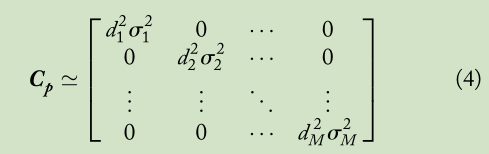
The BLUE for $\theta$ based on (3), denoted by $\hat{\theta}$ , is then [12]

注：我信了你的邪，这个[12]参考的是统计信号处理基础中的估计理论。我还没有去查看这本书的具体解释，看了几篇论文都是直接给出。我且先认为就是如此吧！

where -1 represents matrix inverse. Note that the LSC estimate is given by (5) with the substitution of $\bold{C_p = I_M}$ where $\bold{I_M}$ is the M * M identity matrix, without utilising the mean and covariance of the data. Since $\{d_i\}$ are unknown, they will be substituted by $\{r_i\}$ in practice. The covariance matrix for $\bold{\hat \theta}$ , denoted by $\bold{ C_{\theta}}$ , is [12]

$\bold{\hat \theta}$ 的协方差矩阵，由 $\bold{ C_{\theta}}$ 表示，是[12]

where the variances for the estimates of x and y are given by the (1, 1) and (2, 2) entries of $\bold{ C_{\theta}}$ , respectively. It is worthy to mention that the same weighting matrix of $\bold{C^{-1}_p}$ has been proposed in [14], which can be considered as a constrained weighted least squares calibration (CWLSC) algorithm with utilising the constraint of $x^2 + y^2 = R$ . We expect that the BLUE-LSC algorithm is inferior to the CWLSC scheme as the parameter relationship in $\theta$ is not exploited.

其中x和y估计的方差分别由 $\bold{ C_{\theta}}$ 的（1,1）和（2,2）条目给出。值得一提的是，在[14]中提出了相同的加权矩阵，可以将其视为利用 $\bold{C^{-1}_p}$ 约束的约束加权最小二乘校准（CWLSC）算法。我们期望BLUE-LSC算法不如CWLSC方案，因为 $\theta$ 中的参数关系未被利用。

注：[14]这篇文章的地址为：

BLUE-LLS algorithm

On the other hand, subtracting the first equation of (2) from the remaining equations, R can be eliminated and we get

(M - 1) equations

Expressing (7) in matrix form yields

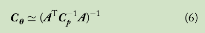
Following the development of the BLUE-LSC algorithm, the BLUE-LLS estimate for $\bold{\Phi}$ based on (8), denoted by $\bold{\hat \Phi}$

where $\bold{C_q}$ is the covariance matrix for q which has the form of

With the use of matrix inversion lemma, its inverse can be computed as

Note that the LLS estimate is given by (9) with the substitution of $\bold{C_q=I_{M-1}}$ ,without utilising the mean and covariance of the data.

The estimator of (9) has minimum variance according to the data model of (8). It is worthy to note that although the dependent variable of R is eliminated in the LLS approach, estimation performance degradation occurs in the conversion of (2) to (7) or (8).

根据（8）的数据模型，（9）的估计量具有最小方差。值得注意的是，尽管在LLS方法中消除了R的因变量，但在（2）至（7）或（8）的转换中发生估计性能降级。

This is analogous to TOA and TDOA-based positioning where the former estimation performance bound is lower than that of the latter if the TDOAs are obtained from substraction between the TOAs [15, 16]. The covariance matrix for $\hat\Phi$ denoted by $C_{\Phi}$ , is

这类似于基于TOA和TDOA的定位，其中如果TDOA是从TOA之间的减法获得的，则前一估计性能界限低于后者[15,16]。用于表示 $\hat\Phi$ 的协方差矩阵 $C_{\Phi}$ 是

注：这篇文章，看到这里大致可以了，下面的的确有点生涉难懂，至于仿真暂时就不仿真了。留着以后有闲心了仿真。

其实BLUE_LLS对我还是挺有启发的，这种启发在于接下来，我做TDOA定位分析有利。因为这个过程，与TDOA神似，这是后话，后面的博文会作出分析。

Although there are at most M(M - 1) LLS equations can be generated from (2), only (M - 1) are independent [10]. In fact, (7) is an example of the independent set of equations.

虽然最多可以从（2）生成M（M - 1）LLS方程，但只有（M - 1）是独立的[10]。实际上，（7）是独立方程组的一个例子。

Although we can use up to M(M - 1) dependent equations in the standard LLS algorithm, this is not possible for the BLUE realisation because the corresponding noise covariance matrix will be singular. In the following, we will prove that as long as the (M 2 1) equations belong to the independent set, the BLUE-LLS estimator performance will agree with the covariance matrices given by (6) and (12). Their suboptimality is then illustrated by contrasting with the CRLB.

虽然我们可以在标准LLS算法中使用多达M（M-1）个从属方程，但这对于BLUE实现是不可能的，因为相应的噪声协方差矩阵将是单数的。在下文中，我们将证明只要（M-1）方程属于独立集，BLUE-LLS估计器性能将与（6）和（12）给出的协方差矩阵一致。然后通过与CRLB对比来说明它们的次优性。

First, we define two sets

where $\Theta$ corresponds to all independent sets of the LLS equations. In doing so, we can generalise (8) as:

其中 $\Theta$ 对应于LLS方程的所有独立集合。在这样做时，我们可以将（8）概括为：

As an illustration, substituting $K = [-1_{M-1},I_{M-1}]$ in (16) and (17), where $1_{M-1}$ is a column vector of length M-1 with all elements equal 1, yield (9) and (12).